Theory
Real World Plots
Working with Polarplot Software
Reference Antenna
Introduction
Recently I received carefully made real world pattern plots of my GTV 2-14w. Which I take as a call to discuss
the ever smouldering topic of whether NEC produced antenna patterns do match with real word results.
When I started investigating Yagis, doing own designs and Boom Corrections I found backup and references
in both SM5BSZ and DL6WU/DJ9BV findings which I explain down this page.
SM5BSZ abt. the measurements taken at the Nordic VHF Meeting Öland 1996.06.06
mentioning the Difficulties plotting Yagis on a test range
" We want to have information about fields down to 40 dB below the field in the forward direction.
With a conventional setup this is not easy (understatement). Very high towers would be needed.
(...) Houses, trees and other objects have to be far away to not produce reflections above the -40 dB level."
Leif Åsbrink, SM5BSZ on http://www.nitehawk.com/sm5bsz/oland/index.htm
It is understood that if we want to achieve a measurement accuracy well below -30 dB or even -40 dB against the normalised
directive antennas gain in forward direction, we need to measure in an environment that reflects less than that
by many dB's.
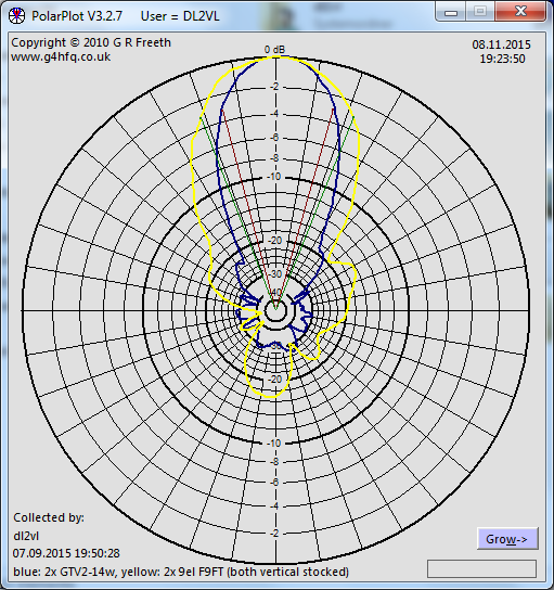
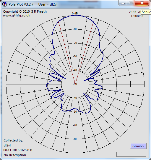
A plot sample showing two Yagi arrays overlayed on courtesy of Jörg DL2VL
(PolarPlot V3 by G4HFQ)
How many OMs have been looking up this website?
Fundamentals
An ideal Far Field plot can only be produced at an infinite distance between the transmitting and receiving antennas.
This is because only then is a plane wave front presented to the AUT. In practical terms (due to the curved nature
of concentric wave fronts) only at a large distance is the phase lag marginal at the illuminated far ends of the
aperture area of the AUT.
Extracted from "Cand.-Ing. Joormann, University of Duisburg/Esssen:
Einrichtung eines Antennenmesssystems für sogenannte Fernfeldmessungen"
Phase lag errors lead to
• filled nulls, increased side lobes
Amplitude errors lead to
• possible decrease of side lobes, ripples in plot line
Sampling errors lead to
• angle diversions, filled nulls
The AUT must be turned around its Phase center (usually the driven element) or plot holds
• phase-, amplitude- and angle errors
A reminder of what -40 dB means in linear quantities ...
Challenges to master for achieving deep nulls and produce a correct plot down to -40 dB of F/B or F/R
• 0 dB equals a numeric factor of 1
• 10 dB equals a numeric factor of 10
• 20 dB equals a numeric factor of 100
• 30 dB equals a numeric factor of 1,000
• 40 dB equals a numeric factor of 10,000
but
• -20 dB equals a numeric factor of 0.01
• -40 dB equals a numeric factor of 0.0001
If we want to measure with correct results down to -40 dB we need feed our transmitting probe antenna with a suitable
constant output level. For a given 1 W we need to meet a consistency in the 0.0001 W = 100 uW range to achieve that.
On the RX side we must perform linear processing of the signal down to at least -40 dB as well in order to render our
pattern plot correctly.
DL6WU / DJ9BV's Expert Knowlegde
The following is a key citation taken from a set of 4 article series by Rainer Bertelsmeier, DJ9BV and Günter Hoch, DL6WU
Bertelsmeier R., DJ9BV, Hoch G., DL6WU: Yagi Simulation: CAD-Software for Evaluation and Development - Part II, Dubus 4/1991
"Test Range Measurements
Unless special precision is required (like callibrating a gain standard) antenna measurements are made
acccording to EIA 136. This standard imposes bounds on diverse parameters, e.g. on field homogenity:
the field must not vary by more than 0.5 dB [meaning reflections < 0.5 dB] thoughout the rotation volume
of the device under test [the AUT]. You will hardly find an amateur test range where this basic condition is
met. - or even checked. From own experience we estimate the accuracy of a good professional outdoor range
measurement as follows:
Gain (...) +/-0.2 dB
Beamwidth and positions of nulls or minor lobes +/-0.5 dB
Amplitude of side and back lobes 0..10 dB down +/-0.5 dB
10..20 dB down +/-1 dB
20..30 dB down +/-3 dB
Anything more than 30 dB below the main lobe [ref. to. normalised pattern] is sheer guesswork."
Error estimation / Fehlerabschätzung
To give an idea about how an error indication looks like mathematically I line out some basics here
The absolute error of measurement is the total differential of the representing function by all measurands /
Der absolute Messfehler ist das totale Differential der Funktion nach allen Messgrössen.
dB_refl       = Grade of maximum reflections on the measurement site/field
dBm           = Constancy of Transimitters output level during plot session
dB_out        = NF output of used Receiver
dB(Degr_slot) = Match of Rotators pointing to a certain degree while Plot-Software assumes a certain angle.
dB_lin        = Linearity of Soundcard that processes the signal level from receiver to plot-software
dB, Plotchart = Linearity of plot-softwares input to chart
For a minimum these terms line up to the total measurement error when doing a real world pattern plot.
Of coarse all those single functions ∂ dB_refl with the variable ∂ Field_lin, and ∂ dBm with variable ∂ TX_P_out etc.
will have to be filled in with suitable terms describing these effectively before entering a calculation.
If the tributions are: example wise dB_refl = 2.5 dB, by dBm = 0.1 dB(m), dB_out_RX = 0.2 dB, dB_Degr_Slot = 0.5 dB average, dB_lin_Soundcard = 0.1 dB and
dB_lin_Plotchart = 0.1 dB ... we end up with an absolute measurment error of
Δ dB_plot = 2.5 dB + 0.1 dB + 0.2 dB + 0.5 dB + 0.1 dB + 0.1 dB = 3.5 dB
PolarPlot Software
PolarPlot V3.2.7 Software by G4HFQ
• 50 dB 'dynamic range'
• Logarithmic & linear plots
• Plots overlaying function
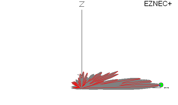
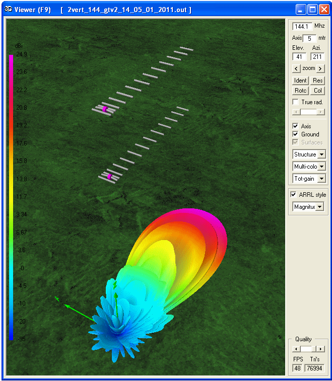
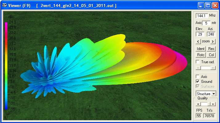
The Real World Plots (1) 2 x vert. stacked GTV 2-14w
Antenna under Test (AUT) is a 2 x vertically stacked GTV 2-14w
Lower Yagi is 16.1 m AGL, upper is 19.9 m AGL - which is 3.82 m of stacking distance
per DL6WU formula
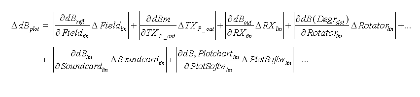
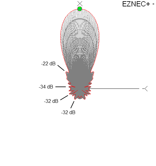
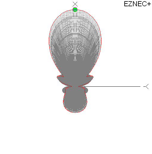
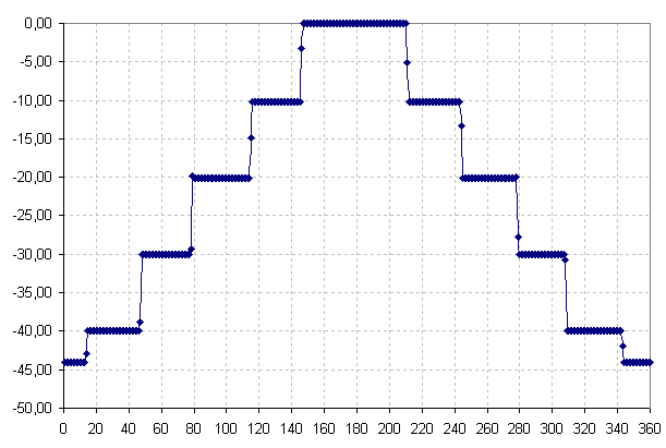
The AUTs EZNEC 5+ simulated azimuth plot in free space
The AUTs azimuth plot @144.200 MHz using PolarPlot V3.2.7 by Jörg, DL2VL

The Real World Plots (2) 2 x vert. stacked Tonna 9 ele. portable version
Antenna under Test (AUT) is a 2 x vertically stacked Tonna 9 ele. (portable version)
Lower Yagi is 12.0 m AGL, upper is 14.8 m AGL - which is 2.77 m of stacking distance
per Tonna manual
UR5EAZ abt. calculation of Forward Gain
From the Helpfile for Polarplot V3 by Bob, G4HFQ
"For its calculations the program uses particular ratios between the horizontal and vertical
beamwidths based on the number of elements. The difference between horizontal and vertical
beamwidth is usually greatest with a 2 element beam, and decreases as the number of elements
increases. When the number of elements is greater than 8 both beamwidths are, for practical
purposes, the same.".
see here for more
Vladimir, UR5EAZ, in USSR magazine 'INFOTEH HF & UHF REVIEW, March 1990:
UR5EAZ's MS Excel table: E_nec = E plane HPBW, H_nec = H plane HPBW

Handling the raw data plot file
The PolarPlot data file '.plp' format is a non binary, simple numbers file. Hence it is easy to read and use for own applications apart from or inside PolarPlot.
A .plp file opened in Notepad++
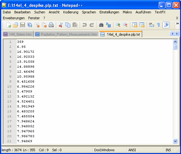
.plp File Format in Detail
1 = Highest reading number // total plot lines
2 = plot line values per tick
...
...
...
n = last plot line value
n + 1 = Number of readings to plot for 360 degrees
n + 2 = Trim End // represents possible end of lines to plot from in case of file in excess of 360 ticks
n + 3 = Rotation angle in degr. // for rotating the whole data set in a displayed chart
n + 4 = Peak dB Down Observed //  for issuing a warning about a peak level higher than sound cards max. output
n + 5 = Trim Front // represents possible start of lines to plot from in case of file in excess of 360 ticks
n + 6 = Start of File Description and Polarplot Vers.
....
Details above are provided by G4HFQ. Thank you Bob!
Reading this file into MS Excel, converting numbers by converting to dB log and normalising (peak gain as zero)
leads to valid pattern charts
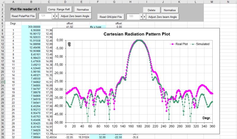
Compare with PolarPlots chart in carthesian coordinates, log. scaling (plot by DL2VL)
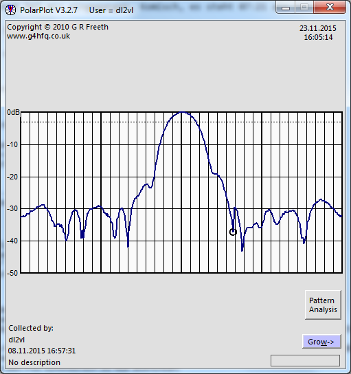
Compare with PolarPlots chart in polar coordinates, linear scaling (plot by DL2VL)
PolarPlot File Format Handling Numbers and Constants
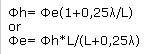
Conversion of raw data values to dB
20 x log10 ((Raw / 4.00) ) = dB
The data set needs ot be normalised to produce a pattern chart as we are used to.
Which means to find the highes numbers delta to zero dB and subtract that difference form the whole lot.
More about pattern plots see here
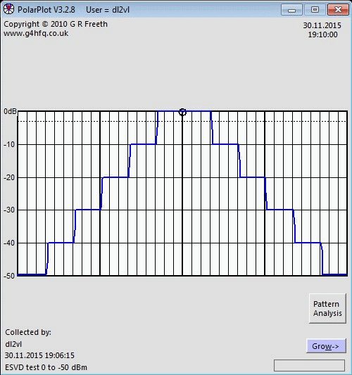
Linearity & accuracy check
... of Polarplot & MS Excel formular and 14 bit AD converter of a Rohde & Schwarz ESVD Test Receiver as
Frontend to Polarplot. Polarplots .plp files raw data converted using 20 x log10 ((Raw / 4.00) ) = dB as a chart
Plotting & equipment provided by Jörg, DL2VL
in dB
   0 =  -0.02
 -10 = -10.21
 -20 = -20.11
 -30 = -29.98
 -40 = -39.95
 - - - - - - -
 -45 = -44.06   out of specs of the R&S
... and down to -50 dB now with PolarPlot v.3.2.8:
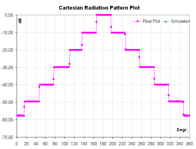
Linearity check (Plotting & equipment: Jörg, DL2VL)
and MS Excel data handling
   step / raw .plp data / actual dB

   0 dB := 1000.0000   =   0.00 dB
 -10 dB :=  309.6448   = -10.18 dB
 -20 dB :=   99.11366  = -20.08 dB
 -30 dB :=   31.74437  = -29.97 dB
 -40 dB :=   10.02587  = -39.98 dB
 -50 dB :=    3.318471 = -49.58 dB
 -60 dB :=    1.299212 = -57.73 dB
Pilot Build of a Reference Dipole for measuring Reflections of Test Range
A Reference Dipole built by Jörg, DL2VL (click on image to enlarge)
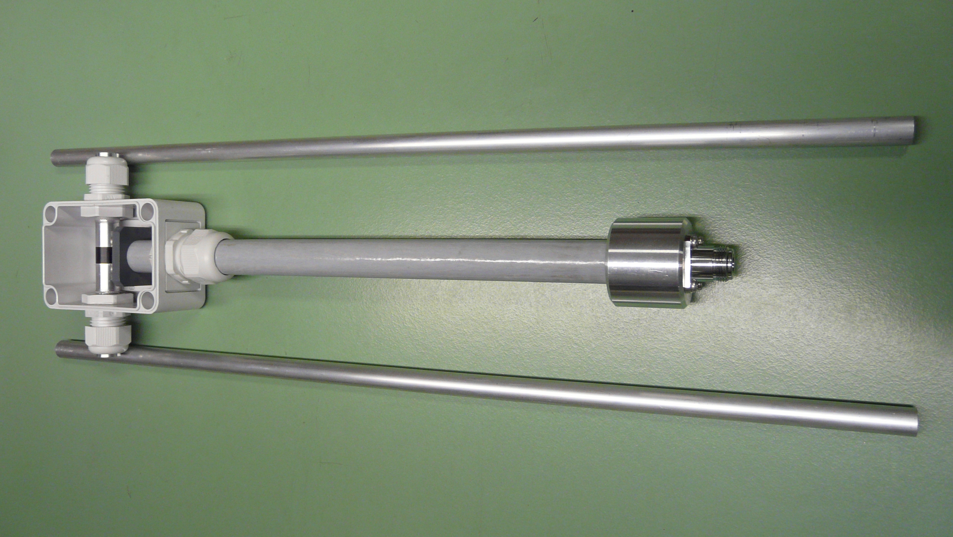
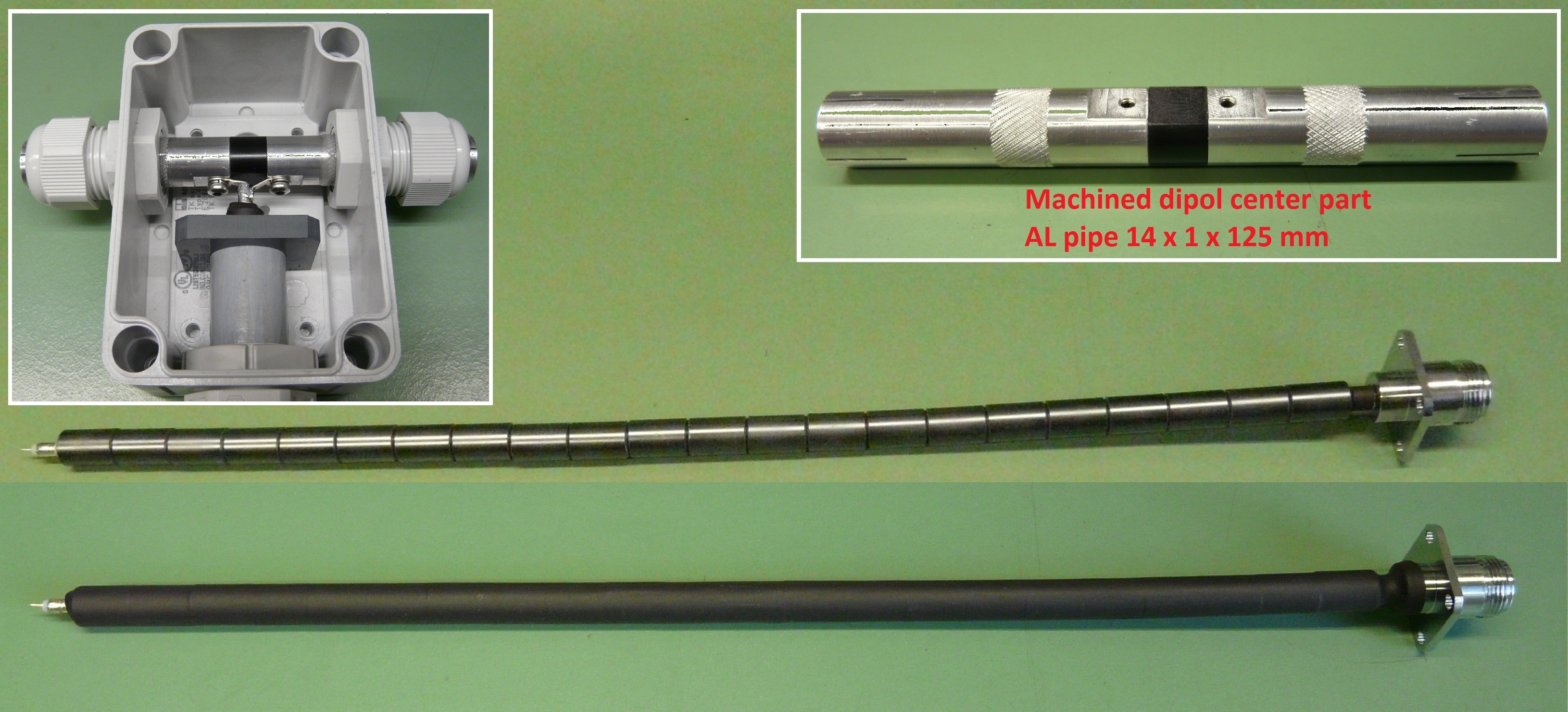

Tnx Jörg!
73, Hartmut, DG7YBN