Basic Coordinate Schemes
Plot Variations using Polar Coordinates
Reading data from a pattern plot
Pattern plots using Cartesian Coordinates
Preface
There are many ways to plot a pattern. The same pattern can look this way or that by how the x and y-axes are scaled. Both show gain in specified angle (Theta = θ, Phi = φ), but scaling these axis can be linear, logarthms or double logarithmic.
Numbers plotted can refer to the antenna pattern numbers directly (non-normalised) - or be normalised to the maximum gain as zero so that likewise 16.2 dBi equals 0 dB.
An F/B of -17.1 dB attentation against the main beams (+)16.2 dB equals normalised -33.3 dB. Using normalised gain enables us to read the delta between expected signal reading from beam direction and others in direct numbers.
Testing a Yagis directivity by turning to a beacon and next turning by 180 degrees reading the F/B we expect 5 and a half S-units in difference on the shown model. The normalised plot delivers that in same "look and feel" right away.
The non-normalised plots shows that too, but we have to sum up the span from +16.2 dB(i) of forward gain to -17.1 dB in rear direction to the -33.3 dB attenuation to derive the behaviour the Yagi will show when observing the S-meter.
The decibel (dB)
... is the tenth of a bel (Alexander Graham Bell) ... is a logarithmic unit (full stop). When discussing ARRL and non-ARRL plot styles we have to remember that the decibel is logarithmic already. If we press that into a logarithmic scale it will appear as double logarithmic in the charts plotline.
Plot Schemes - Polar and Cartesian Coordinates
Any plot style holds a convention, how a dot in field or space shall be identified: 2D polar plots use an angle and a length. 3D polar plots need two angles (θ, φ) and a length. The Cartesian plot is the "common" plot with x and y coordinates.
The first image shows the full 3 dimensional plot. For any Yagi "build" along the x-axis as boom and horizontal polarisation the flat circle pierced by x- and z-axis referes to the elevation plot (H-plane). The lying circle pierced by x- and y-axis referes to the azimuth plot (E-plane).
• 3D Polar Plot
In order to show the context details clearer the following images hold 2 dimensional information only. Picking the flat circle that referes to the elevation plot only, the difference between linear (on left) and logarithmic scaling (on the right side) of the two axis carrying the gain numbers is shown.
• 2D Polar Plot, gain as linear dB scale • 2D Polar Plot, gain as logarithmic dB scale
If we "cut" the circle and roll out its circumference, we transform the polar plot into Cartesian coordinates.
• Cartesian Plot (with linear gain on upright axis)
ARRL Style & Normalised Pattern Chart - using Polar Coordinates
Normalised View - means max. gain is set to 0 dB(i) as plotted on Y-axis. All other data like F/B refer to zero here. An F/B of -18.0 dB means if we adjust a meter to zero when pointing the main beam directly into source direction we will lose -18.0 dB on it when turning the antenna by 180 degrees. In S-meter units we find it attenuated by 3 units then.
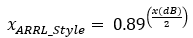
ARRL Style means gain displayed on a logarithmic scale of 0.89 times the value of the signal voltage.
Quote Dan, AC6LA: Coordinate Scales for Radiation Patterns
"ARRL Log Coordinate System
The modified logarithmic grid used by the ARRL has a system of concentric grid lines spaced according to the logarithm of 0.89 times the value of the signal voltage. [...] For example, the scale distance covered by 0 to -3 dB is about 1 / 10 of the radius of the chart. The scale distance for the next 3 dB increment (to -6 dB) is slightly less, 89% of the first, to be exact. The scale distance for the next 3-dB increment (to –9 dB) is again 89% of the second. The scale is constructed so that the progression ends with -100 dB at chart center."
• Azimuth plot ( = E-plane for any horizontly polarised antenna)
• Elevation plot ( = H-plane for any horizontly polarised antenna)
How to produce your own chart:
For normalised data in dB per angle we may use this formular:
In MS Excel (TM):
Insert a Radar Chart (Netzdiagramm) > values: gain through 0 ... 360 deg.,
axis settimgs: range 0.0 ... 1.0, linear = non log. scaling of value axis, no labels on value axis
Now we need a reverse pointing log. scale for the value range, which spans from 0 to -50 or -100.
However the logarithm will only work out with positive values entered. So in the end we set a background image into the chart which shows 0 dB to -50 dB were the real values span is 1.0 ... 0.0.
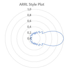
• ARRL Style Plot Chart Background Image
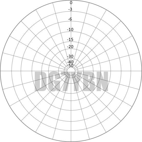
GTV 2-14w (same Yagi as in examples above) in own ARRL style polar chart pattern plot in MS Excel (TM)
Non-normailsed ARRL Style-Gain-as-log
No normalisation - means max. gain is plotted on Y-axis
ARRL Style but no normalisation - means max. gain is plotted on Y-axis
• Elvation plot
Normalised with "linear" Gain
Normalised View - means max. gain is set to 0 dB(i) as plotted on Y-axis
No ARRL Style- means gain is plotted as linear scale ...
which means that small side lobes will appear smaller whereas larger lobes will appear larger compared to the common ARRL-style plot. In this case, with back lobes down to -33.3 dB (against main beam gain as "0" i.e. "normalised") we hardly see anything going on on the rear side of this Yagi. So the "Normalised" or even "Not-Normalised" "Non-ARRL-View" is less suitable for judging or developing antennas with a high directivity factor.
• Elvation plot
Reading the F/B ratio from a pattern plot
As the F/B is similar in both E- and H-plane we need to look at one plane only. Usually the H-plane tells most we need to know.
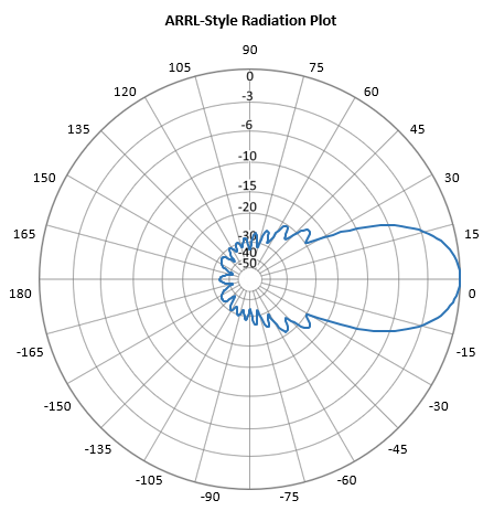
• Normalised ARRL Style
Gain in beam direction is normalised to "0", when turning the antenna we yield a loss in signal strength by -33 dB in free space conditions.

• Non normalised ARRL style
This time gain in main beam direction is not normalised. It is at 16.2 dBi, mind the scaling of the gain axis. Gain in rear direction is -17.1 dB. The difference between both is what we have to expect as loss in signal strength now.
F/B = -17.1 dB(i) - 16.2 dBi = -33.3 dB

Reading the F/R ratio from a pattern plot
As the H-plane produces the larger side- and backlobes usually (for any Yagi and their derivates) we concentrate on that one only.
• Normalised ARRL Style
Gain in beam direction is normalised to "0". When turning the antenna so that the signal strength is maximum of what we find in the entire rear sector we yield a loss in signal strength by -28.3 dB in free space conditions.
• Non normalised ARRL style
This time gain in main beam direction is not normalised. It is at 16.2 dBi, mind the scaling of the gain axis. Maximum Gain in the rear section is -12.1 dB. The difference between both is what we have to expect as loss in signal strength now.
F/R = -12.1 dB(i) - 16.2 dBi = -28.3 dB
Note: There are many ways of how the F/R is defined. Above I use the way that Ari Voors uses it in 4nec2 and VE7BQH uses it in the G/T tables. A more complex definition is to integrate over all lobes and minimum magnitudes using a constant delta angle over the back section and produce a mean number, which is laborious and does not show any high peaking lobes influence if these are 'hit' by unwanted noise.
Reading the 1st side lobe from a pattern plot
• Normalised ARRL Style
Gain in beam direction is normalised to "0". When turning the antenna so that the first sidelobe picks up the signal we yield a loss in signal strength by -17.4 dB in free space conditions.
Reading the sidelobes magnitude from the non-normalised plot works thru applying similar maths as in the examples above.
Rectangular Cartesian Coordinates Plot
• Normalised ARRL Style
What has been displayed in polar coordinates above can also be plotted in "standard" cartesian coordinates. The red stripe from left to right markes the F/B. Basically there is no other information hidden in this way to plot a pattern. It is just an other way to put the numbers on a chart.
But the back lobes are visibly larger to notice.
Max. Gain is in the middle at 0 degrees; Backside ends at 180 respectively -180 degrees left and right side.

73, Hartmut, DG7YBN