In general about EZNEC, 4nec2, MMANA and others Sample of how front-end and kernel work together / 4nec2 EZNEC / Same show, different front-end Xnec2c / Different front-end, Unix/ Linux based MMANA-GAL Basic / Same show, different front-end, mininec kernel
Add-On's for Antenna Temperature & G/T computing
Program RFNC for Evaluation of G/T and more New Program AGEC for Evaluation of Antenna Efficiency New Online AGTC for Antenna Temperature from EZNEC & 4nec2 FFTab-files New Program TANT for EZNEC & 4nec2 Program TANT - Unusual Application by UR5EAZ Program Noise.exe for MMANA-GAL
Convergence challenge
Convergence problems and AGV correction per KF2YN
Model Segmentation
What the NEC2 manual says about wire segmentation
Miscellaneous
4nec2 & GNUplot installation and how to fetch data for use in MS Excel How to fetch data from MMANA for use in MS Excel Some links regarding the topic NEW
Display all content opened
Antenna Modelling and Analysing Software
Preface
This website shall give newbies to antenna modelling an overview on the most frequently used programs.
But I also show a few details that are essential for a deeper understanding and correct judging of antenna
models setup and properties verification that are not included in everybodies standard repertoire.
The big 3 in ham antenna modelling software are EZNEC, 4nec2 and MMANA-GAL. Apart from these there are
YO, AO and also NECWin Plus, NEC2GO.
There are other, non nec or mininec kernel based programs. And other EM (electromagnetic modelling) software
based on 'mesh engines' such as FEKO EM, Ansys HFSS, Sonnet EM which do cost a pretty buck.
It must be mentioned that the commercially discontinued AO Antenna & YO Yagi Optimizer by K6STI due to its
features handling tappered wires, mounting brackets, optimiser and wires meeting at angles (YO only) is a
(not existing any more) option to which many designers who have it stick to. YO models Yagis with straight
elements only, AO models any antenna. Both are DOS screen programs.
I also mention Yagi Analysis by SM2IEV, because in its time it made an impact on the VHF /UHF Yagi
developer scene. As it was and is the only Yagi-Uda antenna modelling software that includes producing
the Antenna_G/T. Though it is not as accurate with Antenna Temperature and G/T as the TANT program
in combination with reading the 3D pattern from EZNEC or 4nec2. Thanks to this feature it gave, lets
call it an early insight view on developing better Yagi stacks for earth-moon-earth operation.
How many radio enthusiasts have been looking up this website since Jan. 2016?
Front-ends to the solving engine: In general about EZNEC, 4nec2, MMANA and others
This chapter is written with a programmers view (I do industrial programming for 6 years now to earn my living).
But I find this approach quite useful to understand how the issued software works, which is the first step to
improved handling of such.
Antenna modelling software based on nec2, nec4, mininec kernels is a front-end to the named kernel.
We could say these softwares are 'User Interfaces' that handle a data set, namely an antenna geometrie and a command
to compute something to the kernel, which does the real work. Finally they handle the kernels output into charts or plots
when the calculation are done.
This is why for instance 4nec2 and EZNEC show the least of marginal aberration when we compare pattern or Return Loss plot output.
Provided both run same setting and kernels, like option 'Use Extended Thin wire Kernel...' (in the nec cards this is line 'EK'.
Which by standard is 'turned on' in both EZNEC and 4nec2. Only when opting for the Standard Thin Wire Kernel the
'EK' line is added to the nec wires card
The kernel is fed with the geometry of an antenna design. In a strictly formatted table.
As the kernel is programmed in Fortran and needs to be fed with commands and parameters according the nec cards
description in the NEC Manual. It is the front-ends task to provide a useful interface like a table calculation like
geometry input or a geometry orientated editor and transform this into the NEC Cards tables before feeding the kernel.
It is understood that the genius of computing the antenna properties lies at the employees of the Lawrence Livermoore
Laboratories that coded the NEC Kernels. But it is also understood that the genuis of providing a convenient human machine
interface lies at the makers of said antenna modelling software. As before that punchcards needed to be produced and
fed to crude computation machines. That is why NEC Cards are called NEC Cards. Because in the beginning they were
hard paper punchcards.
Of coarse it is the same mechanism with mininec based front-ends i.e. antenna simulation software.
Just with some mininec specific details now. Understanding this we see that it does not come down to the
question whether 4nec2 or EZNEC are producing the better numbers, because both use same engine or kernel.
So that their output is identical except possible rounding errors on the very far end of decimal float values
variables the programs are handling.
Sample of how front-end and kernel work together / 4nec2
I have chosen 4nec2 for this first example because in this software we find a separate window for each step of the
'communication' between kernel and user interface = front-end. Which for newbies to 4nec2 might be more
confusing then with EZNEC but can be an advantage for the experienced user, or after having read this acticle hopefully.
Read a step-by-step description how 4nec2 operates the nec kernel
4nec2 main window
(1) The front-ends task to provide a useful editor for the antennas geometry (4nec2 'NEC editor')
(2) Prompting a command to the kernel (4nec2 'Calculate / Generate window')
Here: to compute the Far Field Radiation Pattern
(3) Calling the kernel (button 'Generate')
When doing a computation we see 4nec2 calling up the NEC Kernel through this popup DOS console window.
Which holds a line showing the internal names of the input and output file to and from the kernel
and what kernel (here nec2d) is called up
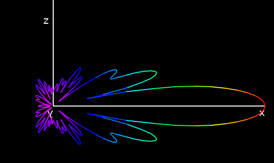
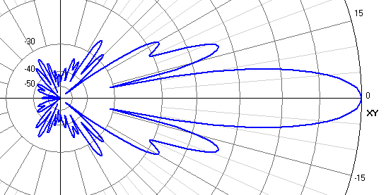
(4) The front-ends task of interpreting the kernels output in a useful way (4nec2 'Pattern' window)
4nec2 is programmed by Arie Voors.
From his website:
"4nec2 is a completely free Nec2, Nec4 and windows based tool for creating, viewing, optimizing and checking
2D and 3D style antenna geometry structures and generate, display and/or compare near/far-field radiation patterns
for both the starting and experienced antenna modeler."
The maximum number of segments, wires, field points, exitations / sources is a virtual one in 4nec2.
The user can edit these settings up to the amount of memory the machine 4nec2 is running on can handle.
The kernel in use has its own limitations too. The standard nec2d & nec2dSX kernels handle max. 11,000 segments.
I can for instance run a 4 bay of 26 element DJ9BV BVO Yagis containing 2236 segments in 132 wires just like that,
engaging the enclosed nec2dXS kernel with max.-No. of nec LD cards set to 256 instead of default setting of 64 cards.
Which the full version of EZNEC v.5 or 6 will not do as they are limited to 500 segments.
There is an online help for 4nec2 holding explanaintions and a number of PDF files.
Amoung these is the 'A Beginner's Guide to Modeling with NEC' by L.B. Cebik, W4RNL, QST Nov. 2000
EZNEC / Same show, different front-end
Read a step-by-step description how EZNEC operates the nec kernel
(1) EZNEC wires window as the front-ends geometry editor
(2) Prompting a command and calling the kernel, the first is integrated into the main window (button 'FF Plot');
the second is running in the background = hidden from the screen
(3) EZNEC plot window as the kernels output interpreter
EZNEC v.5 and v.6 feature the nec2 kernel.
EZNEC is produced and sold by W7EL.
The demo version of EZNEC v.6.0 is limited to handle 20 segments, the full v.5.x and v.6.0 versions up to 500 segments.
There is a pro version, EZNEC Pro (also referred to as EZNEC+) available that handles 2000 segments and uses the nec4 kernel.
Xnec2c / Different front-end, Unix/Linux based
Read a description about Xnec2c and its abilities
Xnec2c by Neoklis, 5B4AZ is another frontend to the nec2 kernel which comes with a few remarkable details:
• Xnec2c is an open source project build around a port of the original NEC-2 kernel from FORTRAN to C:
It supports multi-threaded operation. Current developer Eric, KJ7LNW: " ... we are working on an automatic antenna geometry tuner using the Simplex optimization algorithm."
• Maximum number of wires or segments?
Xnec2c is written in C and uses memory allocation for the segment arrays. So there
is not upper limit to the number of wires or segments other than the capacity (memory) of the computer.
• Resolution of pattern plots?
Maximum resolution for pattern plots is unrestricted. Input parameter for degrees is an arbitrary floating point number.
A resolution of 0.1 deg. works fine.
The editor as a frontend for the Xnec2c kernel:
Wire ends in x,y,z, number of segments, wire conductivity
Output interpreter: A set of plots of my GTV 70-21n as a 4 bay for demonstration:
• xnec2c can read .nec files as produced by 4nec2 and vice versa if minor issues are changed manually:
If there is no EN card at the end of the file. Xnec2c adds this if missing.
EX cards specify an excitation type of 6 which is not acceptable
(max value is 5). I changed it to 0 (voltage source)
Header - Xnec2c .nec file:
	CM --- NEC2 Input File created or edited by xnec2c 3.5 ---
	CM 2m Extended (Double Zeppelin) Yagi
	CE --- End Comments ---
	GW ... etc.
Header - 4nec2 .nec file:
	CM 2m Extended (Double Zeppelin) Yagi
	CE
	GW ... etc.
More about the Xnec2c Kernel
The original NEC-2 kernel by J. Burke of Lawrence Livermore Labs held a minor bug
when the extended thin-wire kernel is used with wires connected to patches because max. number
of Segments (MAXSEG) was 10000, and ICON1 and ICON2 are dimensioned to 2*MAXSEG, so
10000 did not exceed the bound. This is fixed in xnec2c.
The Extended Thin-Wire Kernel can be used as an option (nec wires card entry "EK").
Documentation of Xnec2c and Download:
Xnec2c website: https://www.xnec2c.org/
MMANA-GAL Basic / Same show, different front-end, mininec kernel
pages on a single userform or GUI (Graphical User Interface) in programmer speak. Besides that we find
the same mechanism as with the most spread nec kernel based front-ends EZNEC and 4nec2.
Read a step-by-step description how MMANA operates the nec kernel
(1) MMANA 'Geometry' page as the front-ends geometry editor
(2) MMANA 'Calculate' page
(2) Prompting a command and calling the kernel, the first is integrated into the "Calculate" page (button 'Start');
the second is running in the background = hidden from the screen
(3) MMANA 'Far Field Plots' page as the kernels output interpreter
MMANA features the mininec version 3 kernel. It is brough to you by JE3HHT, DL2KQ and DL1PBD.
The free basic version handles up to 8192 segments or 512 wires.
There is a pro version availabe. It handles 45000 segments, 10000 wires and 300/500 sources, provided you have +16GB RAM
There is an online help for MMANA basic at http://gal-ana.de/basicmm/en/
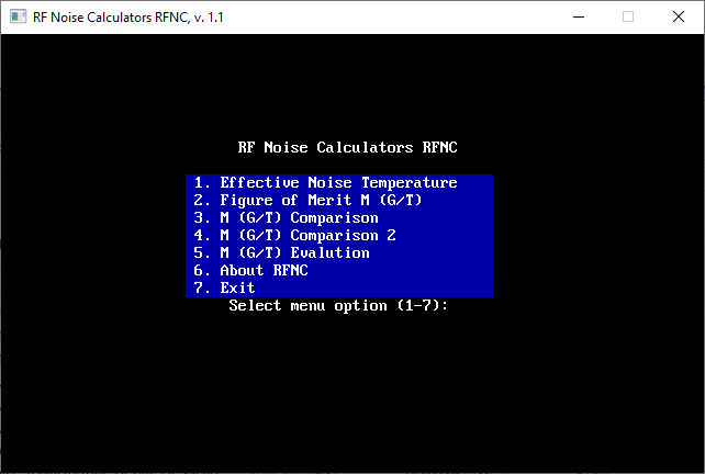
RFNC Program
Posted here: 2026-03-04. Program Version: 1.1, dated 2025-12-06
RFNC runs on any 64 bit windows computer. The program is a single executable file. There's no need to install anything.
The RFNC program has been checked using the VirusTotal tool and does not require installation on 64-bit Windows systems.
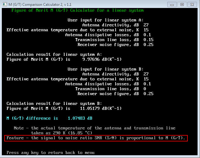
The RFNC is a collection of RF Noise Calculators.
It is written by UR5EAZ.
Feature - for a fixed wavelength, bandwidth and incident power flow density (pfd), the signal-to noise ratio is proportional to M (G/T).
Download RFNC
• Safety Informations:
This is free software.
Liability is therefore excluded to the greatest extent possible. See also
Directive (EU) 2024/2853 Liability for defective products.
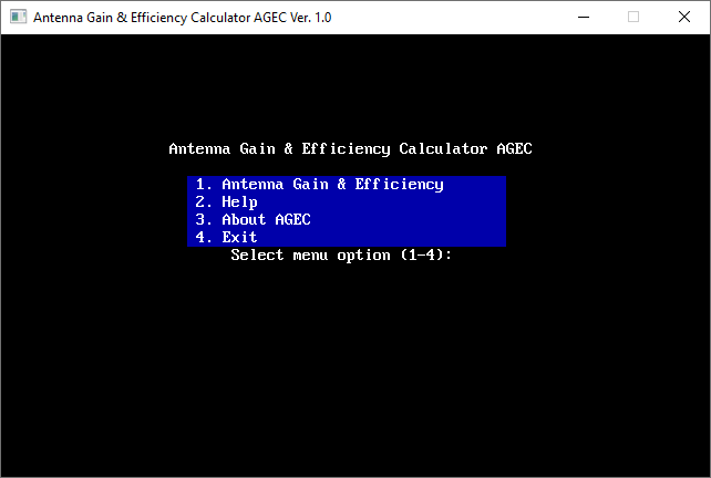
AGEC Program
Posted here: 2026-06-12. Program Version: 1.0, dated 2026-05-31
AGEC runs on any 64 bit windows computer. The program is a single executable file. There's no need to install anything.
The AGEC program has been checked using the Malwarebytes tool and does not require installation on 64-bit Windows systems.
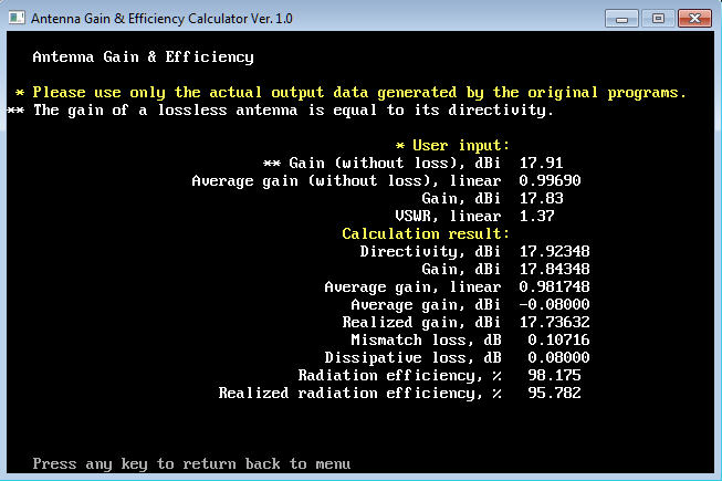
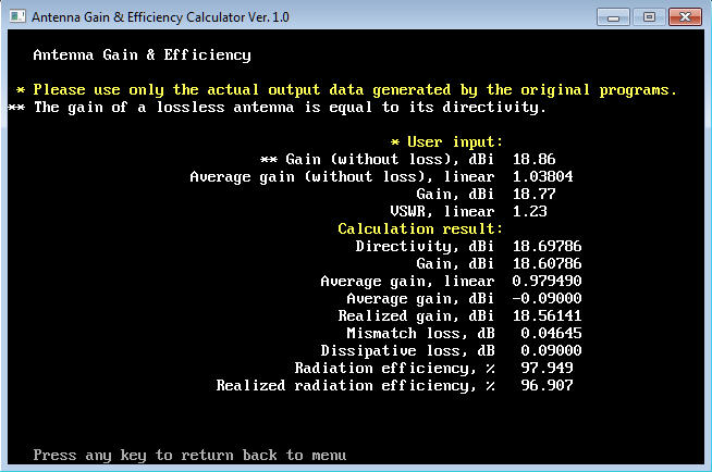
The AGEC is an Antenna Gain & Efficiency Calculator.
It is written by UR5EAZ.
Example 1: Antenna with Average Gain < 1.000:
Example 2: Antenna with Average Gain > 1.000:
Download AGEC
• Safety Informations:
This is free software.
Liability is therefore excluded to the greatest extent possible. See also
Directive (EU) 2024/2853 Liability for defective products.
Online AGTC Antenna Temperature & G/T computing for EZNEC & 4nec2 FFTabs
AGTC-JS_V01-08
• HTML-version of AGTC-2lite; Javascript-based Antenna Temperature and G/T calculation program
The functionality of the QBasic compiled DOS progam AGTC in a single HTML-file web utility.
Link: https://f5fod.github.io/AGTC-JS/ on github
This is a web utility, no need to download.
Javascript is client based, executed local on your computer.
The enclosed javascript will analyse a Far Field Table (FFTab) located on your harddrive.
• Safety Informations:
This is free software.
Liability is therefore excluded to the greatest extent possible. See also
Directive (EU) 2024/2853 Liability for defective products.
Antenna Temperature & G/T computing Program TANT for EZNEC & 4nec2
TANT was progammed by YT1NT, on proposal of YU7EF and with help from YU1CF + YT1NP.
It is small in size a DOS console program that does not need an installation but can be run
from any drive as it is.
Read about the program TANT.exe for Antenna Temperature and - G/T computation from EZNEC and 4nec2 files
most about TANT is described on my website about Antenna Temperature
Read more on how to derive a NEC model for TANT in the official
TANT Manual (PDF)
Read about an 'unusual application' of TANT.exe focusing terrestrial communication by UR5EAZ
Here are 2 applications of TANT produced by Vladimir, UR5EAZ
For any standard application of TANT at zero elevation T_antenna = (Tsky + Tearth) / 2 so that independently of the antennas pattern,
a constant T_ant is the outcome. But what if we tilt the Yagi by 90 degrees of elevation in a theoretical experiment?
Now former T_sky and T_earth become 'T_front_boresight_of beam' and 'T_rear_lobes'. With this change a number of antenna parameters
useful for studying its suitability for terrestrial weak signal communication can be derived. Former T_sky now is the Brightness Temperature
of the sphere that lies in beam direction, while former T_earth becomes the Brightness Temperature of the rear sphere.
(1) The 'Ratio of Radiation Power into Rear Semi-Sphere to Radiation Power into Sphere' MS Excel
This table holds 50, 144 and 432 MHz Yagi-Uda antennas
Download UR5EAZ's MS Excel 'RRF_dB_october.xls'
(the file contains step-by-step instructions)
UR5EAZ produced a second interactive MS Excel table. It shows Antenna and System G/T. In here the user can edit T_earth, T_sky, RX NF and bandwidth
while the numbers for System G/T adapt.
(2) The 'Unusual application of the TANT program' MS Excel
in which T_sky, Tearth and also RX bandwidth and NF can be edited and G/T and System NF are being computed.
This table holds 50, 144, 432 and 1296 MHz Yagi-Uda antennas at an elevation of 5 and 30 degrees
Download UR5EAZ's MS Excel 'INTERACTIVE_TABLE_JANUARY_17.xls' version 2.3
Vladimir likes to thank Lionel, VE7BQH and Hartmut, DG7YBN for consulting and verifying of the calculation
2016-07-05: Vladimir updated his Excel by adding a calculation of expected level of own EME echos when transmitted and received with
a chosen Yagi at a filled in ouput power and RX Noise Figure. A practical number in practise.
Download UR5EAZ's MS Excel 'INTERACTIVE_TABLE_JULY_5_2016_ECHO_SNR' version 2.9
Antenna Temperature & G/T computing Program for MMANA-GAL
Noise.exe is a program developed by Kosta, UR5FFC, 'Black Sea Radio Co.'.
It is a small in size 'windows' program that does not need an installation but can be run
from any drive as it is.
Read about the program Noise.exe for Antenna Temperature computation from MMANA files
It reads files of 3D Far Field plots produced with MMANA
and computes Gain, Forward-, Sidelobe-, Backwards Lobes Temperature and also the conclusive Ohmical Loss and
Antenna Temperatures together with the G/T_antenna. Strictly as described in the well known Article 'Effective Noise
Temperatures of 4-Yagi-Arrays for 432 MHz EME', Dubus 4/87 by DJ9BV.
Download
You can download the PDF manual from my website as a preview.
Click here to call the Download Mirror on my website
• Safety Informations:
This is free software.
Liability is therefore excluded to the greatest extent possible. See also
Directive (EU) 2024/2853 Liability for defective products.
Note: Noise.exe version 1.0 has an internal flaw handling the comma as decimal separator.
If your computers operating system is set to use the "," as default decimal separator you must change to "."
while using noise.exe.
This occure on German settings and maybe on others too.
Call up your Operating systems 'Regional Settings' and change to English
A screenshot of MS Windows 'regional settings' in Ukrainian language and how to change the decimal separator only.
(tnx to Vladimir, UR5EAZ)
Convergence problems and AGV correction per KF2YN
We want 'realistic' antenna simulations. Of such kind, that they can be produced as real antennas.
But the simulation output varies a great deal with the wires segmentation number of the model.
Read about the challenge of getting the models segmentation right
Convergence and Limes,
a simplified mathematical introduction
The strict mathematical definition of convergence is more complex than this Limes or Limit of a function.
But in simple terms we are looking at a sample function f(x), which approaches a Limes, a highest number, towards the value 2.00.
For a certain ε all values of that function are within L = 2 ε from input value S on.
Math.: 'For all x > S the f(x) is within ε of L'.
What does that mean to the antenna designer?
We want 'realistic' antenna simulations. Of such kind, that they can be produced as real antennas
with as close as possible properties to the simulated design. Will the radiation pattern and frequency response
be same as designed? Which way is the model set up the right way and how can that be assured?
The ideal scenario is a design, whose nec geometry could be uses 1:1, maybe with a proven boom correction applied.
What happens when we vary the models segmentation density? Lets look at the YU7EF EF0212 with
wires segmented in 3 different densities:
Frequency response versus segmentation on a DG7YBN 432 MHz YBN 70-5m
We see the point of best Return Loss move by 3.5 MHz while varying the segmentation density and also the Average
Gain approaching a limes. With a segmentation of ~10...15 per wire (= Yagi element) we find a change in the Average Gains
line steepness and a close approximation to the ideal value of 1.000. This may be our L = 2 ε.
For most simple antenna structures, be means of forms or layouts of wires that the used kernel can handle with less divergence
many carefully build and plotted test Yagis with a non metal boom show a relatively good conformity to the simulation
with around 11 segments applied per wire. The desired behaviour shows in the region of change in steepness of the Average Gain
curve line.It must be mentioned that to achieve this a correct length of any applied
symmetrising coax or balun is a necessity.
See here, scroll down to 'Preface ... An example' for a real sample plot
See also here 'How to set up a Measurement Yagi the right way?'
See also here 'The SBC ... a Segmentation Density (Boom) Correction'
For comparing the benchmark parameters of forward gain, F/R, Antenna Temperature and Antenna G/T on an objective base the
Average Gain of the lossless models must be 1.000 or at least 0.998 or so. If one of the design models differs from that
we need to apply a correction on its benchmark parameters. This we call Average Gain Correction. The theory was put up by
Brian V. Cake, KF2YN in Dubus 4/2010.
Most about Convergence problems correction including an online calculator using KF2YN's set of formulas is described on my website
about Average Gain Correction
What the NEC2 manual says about wire segmentation
Read about proper wire segmentation
Numerical Electromagnetics Code (NEC) . Method of Moments
Part III: Users�s Guide, G. J. Burke, A- J. Poggio, 1981, Lawrence Livermore Laboratory
Section II, Structure Modeling Guidelines
1. Wire Modeling
(1) �The main electrical consideration is segment length Δ relative to the wavelength λ. Generally, Δ should be
less than about 0.1 λ at the desired frequency.�
λ = 2.079 m @ 144,200 MHz
0.1 λ =0.1 * 2.079 m = 0.2079 m
A typical 144 MHz Yagi element may have a length of around 0.998 m;
At a segmentation of 10 per wire the resulting segment length is 0.998 m / 10 = 0.0998 m.
That leads to a minimum to chose length factor of 0.2079 m / 0.0998 m = 2.08. In straight words:
a segmentation of only 10 segm./wire is better than double of the recommended minimum per manual.
As we continue reading down the manual we find the following:
(2) �[...] while shorter segments, 0.05 λ or less may be needed in modelling critical regions of an antenna.�
Taking into account 'the minimum to chose length factor' we are still on the side of the recommended solution with just 10 segments per wire.
Even if the exciter straight dipole to D1 zone of a Yagi should be considered a critical region. With complexer geometry exiters than a straight dipole
this will become a different story.
(3) �Small values of Δ / a may result in extraneous oscillations in the computed current near free wire ends [�]. Extremely short
segments, less than about 10E-3 λ should also be avoided [�]�.
10E-3 = 0.001 λ 0.001 * 2.079 m = 0.002079 m
2.079 m / 0.002079 m = 1000
segment length = Δ , wire radius = a
(4) �[�] Δ / a must be greater than about 8 for errors of less than 1%.�
• Here is a sketch I made to illustrate the minimum background
Choosing a common diameter for Yagi elements of 8 mm we arrive at a = 8 / 2 mm = 4 mm
Δ / a = 8 gives us a minimum segment length of ? = 8 * a = 8 * 4 mm = 32 mm.
That equals a maximum segmentation of 998 mm / 32 mm = 31
(5) �With the extended thin-wire kernel, Δ / a may be as small as 2 for the same accuracy.�
Δ / a = 2 gives us a minimum segment length of ? = 2 * a = 2 * 4 mm = 8 mm.
That equals a maximum segmentation of 998 mm / 8 mm = 124
(6) �Unless 2 Π a / λ is much less than 1, the validity of these approximations should be considered.�
2 Π a / λ = 2 Π * 4 mm / 2079 mm = 0,0121
On pg. 125 of the manuals we find an example of a Yagi � like structure, take a look at the chosen segmentation:
(7) �Example of a 12 elem. log peridoc antenna
Total 78 segments, No of Seg/wire 9, 9 ,7 ,7 ,7, 7, 7,5 ,5 ,5 ,5 ,5 �
An other voice
L. B. Cebrik, W4RNL
A Beginners Guide to Modeling With NEC,
Part 4: Loads, transmission lines, tests and limitations,
February 2001 QST:
"Whether we have enough segments of the right lengths is subject to a simple test. Start by running the original model and recording the gain and source impedance.
Then increase the number of segments for each wire by about 50%. Again, record the gain and source impedance.
[...] The level of segmentation at which the
output figures for the model do not change significantly is the minimum level of segmentation for the model. The models are said to converge at this segmentation
level. In some cases, minimum segmentation is satisfactory. In others, especially for antennas having a closed
geometry (like angular loops), the required segmentation level may be higher."
4nec2 & GNUplot : Installation and how to fetch data for use in MS Excel
Read about GNUplot, 4nec2's data exchange and table calculation applications
4nec2 is, speaking in programmer terms 'so open for output', that other programs can read the data sets. Arie Voors even
implemented a space for a forseen link to the free gnuplot chart plotting software. So that we do not solely depend on 4nec2's own
chart output but may use gnuplots abilites to produce plot charts to our like or needs.
Further we can use this door for data exchange (4nec2 plot folder & Plot.txt file) to read data into a table calculation software
for whatever data display, analysis or processing
Wikipedia abt. gnuplot
"gnuplot is a command-line program that can generate two- and three-dimensional plots of functions, data, and data fits"
Link to the gnuplot website
Based on the instructions for using the '4NEC2_PLOT.xls' by Vladimir, UR5EAZ, I have written a PDF introduction, how to install
gnuplot, register it in 4nec2 and produce plot data sets for the above MS Excel application.
Download the 'Extended_Output_from_4nec2_with_GNUplot.pdf'
An application for analysing and comparing antenna key parameters, the '4NEC2_PLOT.xls' by UR5EAZ.
• Power Gain
• Q-factor (based on the formulars that YU1AW uses)
• Antenna Absolute Impedance
• Mismatch Loss to given Z
• Return Loss
• Antenna Efficiency
Download UR5EAZ's MS Excel '4NEC2_PLOT.xls'
How to fetch data from MMANA for use in MS Excel & 'MMANA_Plot' MS Excel sheet
Read about MMANA's data exchange and table calculation applications
MMANA plots data, which are to be displayed on internal charts into a 'plot' folder so that other programs can read the data sets.
We can use this door for data exchange and read data into a table calculation software
for whatever data display, analysis or processing
Vladimir, UR5EAZ has written instructions for using the 'MMANA_PLOT.xls' MS Excel application, also produced by him .
"Отличительные особенности:
расширенный набор
анализируемых
параметров
программных
моделей антенн,
возможность
одновременного
анализа двух
моделей,
упрощенная процедура
формирования загружаемых
файлов"
Download the document 'MMANA_Plot_v2'.pdf' in Russian Language
An application for analysing and comparing antenna key parameters, the 'MMANA_PLOT_v2.xls' by UR5EAZ.
• Power Gain
• Q-factor (based on the formulars that YU1AW uses)
• Antenna Absolute Impedance
• Mismatch Loss to given Z
• Return Loss
• Antenna Efficiency
Download UR5EAZ's MS Excel 'MMANA_PLOT_v2.xls' including 2 examples as zipped file
Links
The Clemson University Vehicular Electronics Laboratory
website on Electromagnetic Modeling Software
A listing of all there is in MoM Software Producers in alphabetic order